Modeling the Stress-Strain Curve
of Confined Concrete Using Ensemble
Machine Learning Models

Alex B. Casilla Gallegos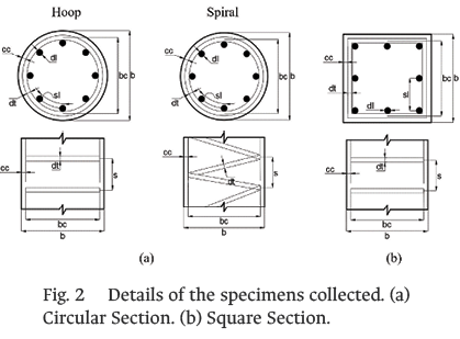

[email protected]

Independent Researcher Civil Engineer

Recibido: 18 Mayo 2025 / Publicado: 24 Abril 2026
https://doi.org/10.26439/ciic2025.8896

ABSTRACT. The objective of this research is to develop an efficient and broadly applicable data-driven model capable of determining the stress-strain curve of confined concrete. Therefore, experimental data of 115 specimens of reinforced concrete columns with square and circular cross-sections were collected from previous investigations in which uniaxial compression tests were performed. Using this data, Random Forest (RF), Adaptive Boosting (AdaBoost), and Extreme Gradient Boosting (XGBoost) models were evaluated to define the most accurate model. Subsequently, the final selected model (based on XGBoost) was optimized, achieving R2 values of 0.97 for the peak stress of confined concrete (ƒcc), 0.93 for the axial strain at peak confined stress (ɛcc), and 0.81 and 0.73 for the axial strains at which stress drops to 85 % (ɛ85) and 50 % (ɛ50), respectively, when evaluated with the testing data. In addition, the SHapley Additive exPlanations (SHAP) technique was used to explain and determine the importance of different parameters in the outcome of the predictive model. Based on the predictions of the XGBoost model, a proposed stress-strain curve was formulated. Finally, a comparison of ƒcc, ɛcc, and the stress-strain curve was performed taking into account the experimental results, the previous models, and the proposed model. The comparison results indicate that the proposed model shows a closer agreement with the experimental data.

Index Terms Confined concrete, ensemble models, machine learning (ML), stress-strain curve.

Thematic Axes Construction processes and new technologies.

Nomenclature

ac	Cross-sectional area of the confined concrete core.
at	Total cross-sectional area.
AC	Area between curves.
b	Dimension of column cross-section.
bc	Dimension of core cross-section.
cc	Concrete cover thickness.
cƒg	Configuration of transverse reinforcement.
dl	Diameter of longitudinal reinforcement.
dt	Diameter of transverse reinforcement.
Dx%	Percentage of predictions within ±x% of the experimental value.
Ec	Elastic modulus of the concrete.
ɛ50	Axial strain at which stress drops to 50% of ƒcc.
ɛ85	Axial strain at which stress drops to 85% of ƒcc.
ɛcc	Axial strain at peak confined stress.
ƒc	Compressive strength of unconfined concrete.
ƒcc	Peak stress of confined concrete.
ƒl	Yield stress of the longitudinal steel.
ƒt	Yield strength of the transverse steel.
FD	Fréchet distance.
MARD	Mean absolute relative deviation.
R2	Coefficient of determination.
RMSE	Root mean square error.
ρc	Volumetric ratio of the longitudinal steel in the cross-section.
ρs	Volumetric ratio of the transverse steel in the concrete core.
Sl	Distance between perimeter longitudinal reinforcements.
St	Spacing of transverse reinforcements (equivalent to s).

1. Introduction

COLUMNS are prone to sustaining inelastic deformations during earthquakes. As a mitigation measure, transverse reinforcement is provided in these structural elements to confine the concrete core, thereby enhancing its inelastic deformation capacity without any reduction in strength.

Given the benefits of confinement, numerous investigations have focused on analyzing the stress-strain curve of confined concrete [1], [2], and [3], to gain a deeper understanding of the material’s structural behavior. However, the main limitation is that these studies propose models that are only moderately useful for very specific specimens, i.e., their range of application is reduced.

The objective of this research is to develop an efficient and general data-driven model to determine the stress-strain curve of confined concrete using ensemble machine learning (ML) techniques. In contrast to mechanical models, the proposed model is applicable to a wider range of cases, reduces error propagation resulting from model assumptions, and provides more information about the stress-strain curve using fewer input data. The development of the model is based on ML, which requires a training process using ensemble models within the framework of supervised learning. The structure of this paper is divided into four sections: model implementation and results, explainability of the final model, proposal of the stress-strain curve, and comparison with previous models.

2. Background

   A. Confined Concrete

The confinement of the specimens is achieved by incorporating transverse reinforcement. This type of confinement is referred to as passive as it becomes effective only when the transverse deformations become significant due to progressive internal cracking. The characteristics of the transverse steel vary according to the shape of the specimen. For circular cross-sections, spiral or circular reinforcement is used, whereas for quadrangular cross-sections, quadrangular reinforcement is used. The benefits of confinement include an increase in maximum stress and improved ductility of the elements [4]. The latter benefit is of great importance for seismic design as greater ductility enables structural elements to withstand higher seismic demands.

B. Ensemble ML Techniques

Predicting the stress-strain curve of reinforced concrete constitutes a regression problem within the category of supervised ML algorithms. Among these supervised algorithms are weak learners and ensemble methods, the latter combining multiple weak learners to enhance the accuracy and efficiency of the predictions [5]. For this problem, three ensemble models were selected, Random Forest (RF), Adaptive Boosting (AdaBoost), and Extreme Gradient Boosting (XGBoost).

The RF model is based on the bagging method, which employs simple parallel algorithms. In this approach, decision trees are trained concurrently, and the model’s final prediction is obtained as the arithmetic mean of the individual submodel outputs [6]. In addition, the AdaBoost and XGBoost models are based on the boosting method, using simple serial algorithms. These models generate new predictors that iteratively correct the errors of their predecessors. However, the models differ in that AdaBoost adjusts the weights at each iteration, giving greater emphasis to erroneous predictions [7], whereas XGBoost adjusts the new predictor to the residual errors made by the previous predictor [8].

C. Performance Metrics

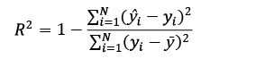
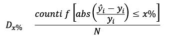
To evaluate the predictions of the outputs, coefficient of determination (R2), root mean square error (RMSE), mean absolute relative deviation (MARD), and Dx% metrics were implemented. This last metric represents the fraction of the dataset for which the relative difference does not exceed a predefined threshold; in this study, a threshold of 10 % was considered [9], [10]. The mathematical expressions for said metrics are shown below:

Where ŷi is the value predicted by the model, yi is the real value, ȳ is the average value of the samples, N is the number of samples, countif is a function that counts the number of data points that satisfy the condition in brackets, and abs is a function that takes the absolute value of its argument.

In addition, two metrics were used to compare the proposed and previous models against the experimental curve: the Area between Curves (AC), which estimates the total area between curves using quadrilaterals, and Fréchet Distance (FD), which quantifies the minimum continuous distance required to traverse both curves [10].

(1)

(2)

(3)

(4)

3. Methodology

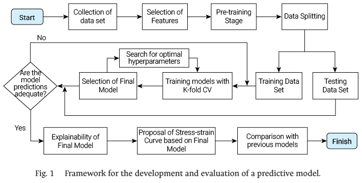
In this research, a framework for developing and evaluating a predictive model is proposed, as illustrated in Fig. 1. The process began with the collection of the data set from previous investigations in which uniaxial compression tests were performed. This was followed by feature selection, a pre-training stage, and the splitting of the data set into training and testing. Subsequently, hyperparameter optimization and K-fold cross-validation (CV) were carried out to select the best performing model. Once the final model was obtained, its predictive explainability was evaluated, and a stress-strain curve was formulated based on its outputs. Finally, a comparison was made with previous models.

4. Model Implementation and Results

   A. Dataset and Selection of Features

The dataset had a total of 115 specimens. The data were extracted from [2], [3], [11], [12], [13], and [14], where they performed uniaxial compression tests on confined concrete specimens. This data set included specimens of normal and high-strength concrete and of square and circular cross-sections, as shown in Fig. 2.

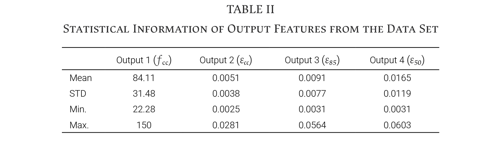
Based on the information collected and the typical design parameters, the final features of the proposed model were defined: six inputs and four outputs. Table I and Table II show statistical information of the features.

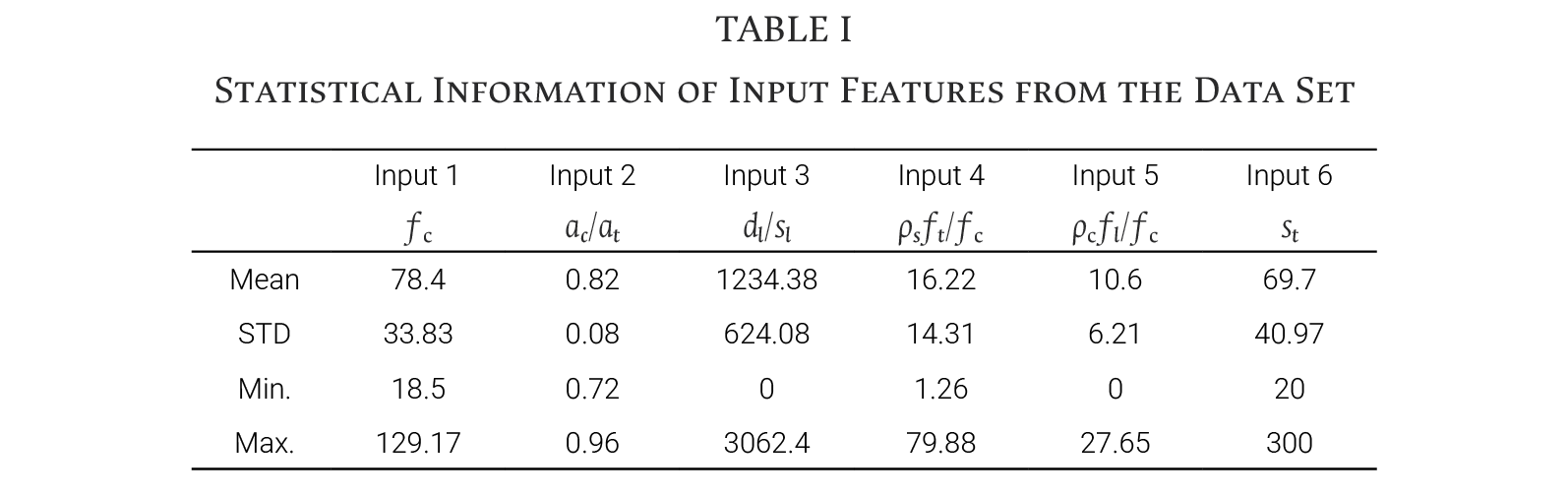
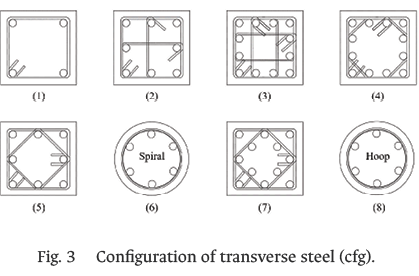
It should be noted that in addition to the aforementioned inputs, the categorical variable input cfg, representing the configuration of the transverse reinforcement, was considered. Within the selected dataset, eight types of cfg were included, as shown in Fig. 3.

B. Model Training and Selection

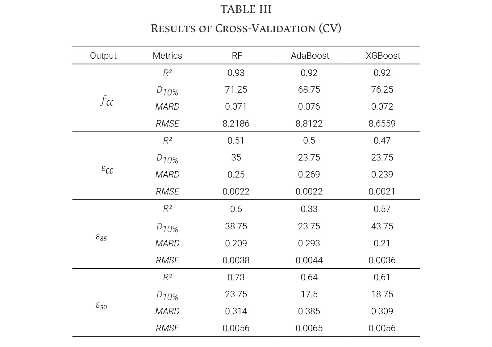
As part of the pre-training stage, the output variables were transformed into logarithmic space to improve data distribution. Feature scaling was also applied to reduce the dispersion of input values. The dataset was randomly partitioned, allocating 70 % for training and 30 % for testing. During the training stage, the three ensemble models—RF, AdaBoost, and XGBoost—were tuned. To prevent overfitting, the K-fold CV technique with five folds was used.

Table III summarizes the performance metrics for each output. Considering all metrics, it is evident that the XGBoost model achieves better results for outputs ƒcc and ɛ85, whereas RF performs best for ɛ50. In the case of output ɛcc, similar results are obtained. In such a way, the RF and XGBoost models present similar global optimal behavior, the latter being slightly better. For the final choice, the XGBoost model was chosen because, in addition to the aforementioned advantages, its greater complexity enables it to handle unbalanced data and categorical variables.

C. Optimization and Validation of the Final Model

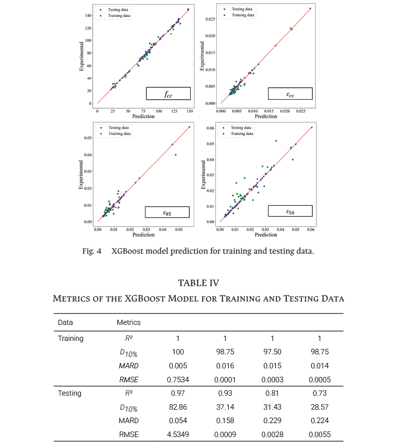
To optimize the hyperparameters of the XGBoost model, the K-fold CV search technique was used. The grid search was conducted using K = 5 for CV. The optimized parameters were: learning_rate [0.1, 0.15, 0.2, 0.25, 0.3], max_depth [2, 3, 4, 5, 6, 7, 8], n_estimators [20, 30, 40, 50, 60, 70, 80, 90, 100, 110, 120]. The results show that the combination of hyperparameters that optimize the predictions is given when learning_rate = 0.2, max_depth = 5, n_estimators = 50. The optimized model was used to generate predictions for both the training and testing data. The graphical results are presented in Fig. 4, and the corresponding metrics are summarized in Table IV. Considering the testing data as unseen by the model, the performance metrics decreased in the following order: ƒcc, ɛcc, ɛ85, and ɛ50. In terms of R2, all four outputs exceeded 0.7, with values of 0.97 for ƒcc, 0.93 for ɛcc, 0.81 for ɛ85, and 0.73 for ɛ50. Thus, the optimized model demonstrates a satisfactory level of predictive accuracy when applied to unseen data.

5. Explainability of the Final Model

The SHapley Additive exPlanations (SHAP) algorithm was used as the primary approach to explain the model. This algorithm is based on game theory to interpret the behavior of ML models [15]. The final model was explained using two complementary approaches: first, through the SHAP Summary Plot, SHAP Dependence Plot, and SHAP Interaction Values; and second, through the SHAP Force Plot.

A. Global Explainability

For the global explanation, the SHAP Summary Plot was used as it integrates both the importance of the input features and their corresponding effects on the model outputs. The results are presented in Fig. 5.

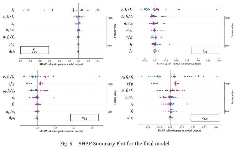
For the output ƒcc, it is observed that ƒc and ρsƒt/ƒc have the greatest impact, whereas for ɛcc the inputs with the greatest impact are ρsƒt/ƒc and ρcƒl/ƒc. In both cases, the mentioned inputs have a positive effect on the outputs.

In the case of the outputs ɛ85 and ɛ50, it is observed that the inputs ρsƒt/ƒc and cfg have greater impact and a positive effect. It should be emphasized that in the case of input cfg the trend does not refer to a numerical value but to the types of cross-sectional configurations shown in Fig. 3. In addition, it is observed that inputs such as ac / at and st have a negative effect since as their values increase the outputs decrease.

Additionally, SHAP Dependence Plot and Interaction Values were employed to relate the output parameters ƒcc and ɛcc to the transverse strengthening index ρsƒt/ƒc and the interaction values. A clear interaction between st and ρsƒt/ƒc was evidenced, as shown in Fig. 6.

Based on these results, it is inferred that as the values of ρsƒt/ƒc increase they cause greater impact on ƒcc and ɛcc. In that sense, it is confirmed that ρsƒt/ƒc has a greater impact on ɛcc, with an approximate maximum SHAP value of 1.5, while for ƒcc the approximate maximum SHAP value is 0.1.

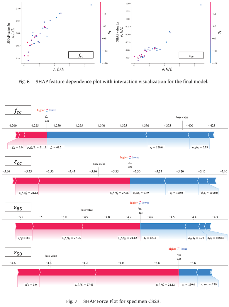
Regarding the interaction, it is evident that as ρsƒt/ƒc decreases, the value of st increases. In such a way, it is determined that the transverse reinforcement ratio is influenced by the transverse reinforcement spacing since as the transverse reinforcement spacing increases the amount of transverse reinforcement in the specimen decreases.

B. Local Explainability

For the local explanation, the SHAP Force Plots were applied for the testing data specimens CS23 and CS16, as shown in Fig. 7 and Fig. 8, respectively. In this manner, we intend to analyze individually the behavior of the inputs over the outputs.

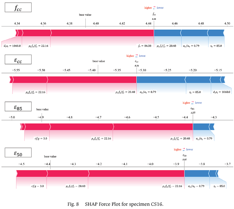
For the output ƒcc, it is observed that higher values of ƒc is high there is a positive impact, whereas lower values produce a negative impact. In both cases, for ɛcc it is observed that ρcƒl/ƒc impacts positively, which evidences the importance of longitudinal reinforcement at the peak point. Finally, in the case of the remaining outputs, the importance of transverse reinforcement is confirmed, as indicated by the positive impact of ρsƒt/ƒc and the negative impact of st.

6. Proposal of Stress-Strain Curve

Based on the outputs of the XGBoost model, a two-branch stress-strain curve was proposed.

A. Ascending Branch

For the ascending branch, the coordinates of the curve peak (ɛcc and ƒcc) of the XGBoost model, and the slopes at the beginning (elastic modulus Ec) and end (zero) of this section were considered. It should be noted that the formulation of Mander (5) was used to calculate Ec.

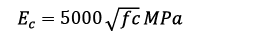(5)

Previous models indicate that a parabolic function adequately fits the experimental ascending curve. However, the Fafitis and Shah (6) approach was adopted for this proposal because it allows the use of all the available information and is not limited to only three data.

(6)

Thus, the formulation (7) was obtained for the ascending branch of the curve.

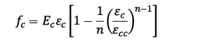(7)

Where:

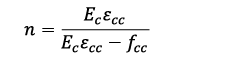(8)

B. Falling Branch

For the falling branch, the coordinates of the curve peak (ɛcc and ƒcc) predicted by the XGBoost model, along with two points corresponding to 85% and 50% of ƒcc were considered. Like the Hoshikuma model, the downward portion of the curve was idealized as a linear function (9).

(9)

However, this proposal differs in that an average slope (mc) was calculated between the slope from the peak point to the point at 85% of ƒcc (mA), and the peak point and the point at 50% of ƒcc (mB). Thus, (10) was obtained for the downward portion of the curve.

(10)

7. Comparison with Previous Models

In this section, two types of comparison were conducted between the experimental results, the previous models, and the proposed XGBoost model. The types of comparison were specific values ƒcc and ɛcc, and the stress-strain curve. It should be noted that among the previous models, Razvi’s model was excluded from this latter comparison because its approach to the curve is identical to that of Mander.

A. Comparison of ƒcc and ɛcc

To ensure a fair comparison, only specimens within the application range of the previous models by Mander, Hoshikuma, and Razvi were considered. Additionally, specimens exhibiting atypical behavior, particularly those with unusually high strain values, were excluded. As a result, the comparison was carried out using 80 specimens, as shown in Fig. 9 and Fig. 10. It should be noted that the vertical axis represents the experimental results from previous investigations, while the horizontal axis shows the predictions from both the mechanical models and the proposed model. The corresponding performance metrics are presented in Table V.

In general, the results of ƒcc are evidently more accurate than the results of ɛcc, across all models. Within the mechanical models, it is observed that predictions of ƒcc by Razvi show better accuracy; while predictions of ɛcc by Mander provide a better fit. In the case of the XGBoost model, the predictions exhibit superior performance compared to all other models, with R2 and D10% values greater than 0.9 and 80, respectively.

Regarding Fig. 10, it should be noted that the mechanical models exhibit increasing dispersion as the strain level rises. This is due to mathematical simplifications and idealizations that do not accurately represent the actual behavior of confined concrete at high-strain levels. In contrast, the proposed model shows reduced dispersion, which is attributed to the inclusion of a sufficient number of high-strain specimens in the training dataset.

B. Comparison of Stress-Strain Curve

For the curve comparison, four specimens, included in the testing dataset, were considered. Among the evaluated models, Mander’s model employs a single expression, whereas Hoshikuma’s model and the proposed model use two expressions to represent the complete stress-strain curve. The results of the curve modeling are shown in Fig. 11. For an accurate interpretation of the curves, the AC and FD metrics were used. The corresponding results are shown in Table VI.

Among the previous models, it is evident that Hoshikuma’s model provides a closer approximation to the experimental curve for specimens SF1P3Y3, CS12, and SS3; whereas Mander’s model performs better for specimen CC21, as Hoshikuma’s approach overestimates the peak-point coordinates. For the proposed model, a strong graphical agreement with the experimental curve is observed when compared with the previous models, as evidenced by the low AC and FD values obtained for all four specimens.

The major differences between the models originate in the descending branch of the curve, where Mander’s model exhibits a notably shallow slope compared to the experimental data, whereas Hoshikuma’s model and the proposed model display behavior more closely aligned with the actual response. This behavior is attributed to the fact that Mander’s model defines the descending branch without incorporating any reference points from that portion of the curve. Although both the Hoshikuma model and the proposed model define a linear function for the descending branch, the proposed model offers an advantage because its slope is derived from two points on the descending portion by averaging the corresponding local slopes.

8. Conclusions

This research proposed the development of an ML model to predict ƒcc, ɛcc, ɛ85 and ɛ50 of the stress-strain curve, and subsequently to model the entire curve using (7) and (10). To develop the model, a total of 115 confined concrete specimens were collected and used to train the RF, AdaBoost, and XGBoost models. Based on the CV results, XGBoost was selected as the final model. Subsequently, the final model was optimized by grid search. In addition, SHAP was used to provide both global and local explanations of the final model. Considering the outputs of the final XGBoost model, a stress-strain curve was proposed. Finally, the predictions from the proposed and the previous models were compared against experimental data.

To begin with, the pre-training stage plays a critical role in obtaining results. Therefore, it is recommended to transform the outputs into logarithmic space, which improves the distribution of the collected information, and apply feature scaling, which reduces the dispersion of the inputs. As shown in the CV results, the XGBoost model performs better than the RF and AdaBoost models.

During the optimization process, the following hyperparameters were selected: learning_rate = 0.2, max_depth = 5, n_estimators = 50. The predictions with the optimized model from the testing data demonstrate favorable results. In terms of R2, all four outputs exceeded 0.7, with values of 0.97 for ƒcc, 0.93 for ɛcc, 0.81 for ɛ85, and 0.73 for ɛ50.

In the model explanation, it is evident that the output ƒcc is highly influenced by ƒc, and ɛcc is highly influenced by ρsƒt/ƒc and ρcƒl/ƒc. In the case of ɛ85 and ɛ50, the parameters ρsƒt/ƒc and cfg have greater impact. Unlike all parameters, ac/at and st have an opposite effect since as their values increase, the outputs have a negative impact. Furthermore, it is observed that when ρsƒt/ƒc decreases, the value of st increases.

Additionally, the XGBoost model achieves better performance than the previous models for ƒcc and ɛcc. Also, in the curve comparison, it is observed that the proposed model shows a high degree of similarity to the experimental curve compared to the other models as it provides a more accurate prediction of the peak point and of the curve’s slope or decay rate.

Furthermore, the developed model has a broad range of applications. Its predictions are applicable to both normal and high strength concrete specimens, whether square or circular in shape, and can accommodate up to eight variations in transverse reinforcement configurations. It is important to note that the input values for the specimens must fall within the minimum and maximum limits of the dataset, as shown in Table I.

Regarding the dataset, it was collected from previous research. However, having experimental data generated specifically for this study would have been advantageous, as it would not only have increased the available data volume but also influenced the selection of the model inputs and outputs.

Finally, future research should focus on integrating hybrid approaches that combine data-driven models with physical constraints, which could improve both the interpretability and reliability of the model for structural design applications.

References

[1] A. Fafitis and S. P. Shah, “Lateral Reinforcement for High-Strength Concrete Columns,” in ACI Special Publication SP-87, High-Strength Concrete, American Concrete Institute, Farmington Hills, MI, USA, Sept. 1985, pp. 213–232.

[2] J. B. Mander, M. J. N. Priestley, and R. Park, “Theoretical Stress-Strain Model for Confined Concrete,” Journal of Structural Engineering, vol. 114, no. 8, pp. 1804–1826, Sep. 1988, doi: https://doi.org/10.1061/(asce)0733-9445(1988)114:8(1804)

[3] J Hoshikuma, K. Kawashima, K. Nagaya, and A. Taylor, “Stress-Strain Model for Confined Reinforced Concrete in Bridge Piers,” Journal of Structural Engineering, vol. 123, no. 5, pp. 624–633, May 1997, doi: https://doi.org/10.1061/(asce)0733-9445(1997)123:5(624)

[4] R. Park and T. Paulay, Estructuras de Concreto Reforzado, 2nd ed., Mexico City, Mexico: Limusa, 1983.

[5] A. Géron, Hands-On Machine Learning with Scikit-Learn, Keras, and TensorFlow, 2nd ed., Sebastopol, CA, USA: O’Reilly Media, 2019.

[6] L. Breiman, “Random Forests,” Machine Learning, vol. 45, no. 1, pp. 5–32, Oct. 2001, doi: https://doi.org/10.1023/A:1010933404324

[7] Y. Freund and R. E. Schapire, “A Decision-Theoretic Generalization of On-Line Learning and an Application to Boosting,” Journal of Computer and System Sciences, vol. 55, no. 1, pp. 119–139, Aug. 1997, doi: https://doi.org/10.1006/jcss.1997.1504

[8] T. Chen and C. Guestrin, “XGBoost: A Scalable Tree Boosting System,” Proceedings of the 22nd ACM SIGKDD International Conference on Knowledge Discovery and Data Mining - KDD ’16, vol. 1, no. 1, pp. 785–794, Aug. 2016, doi: https://doi.org/10.1145/2939672.2939785

[9] X. Guan, H. Burton, M. Shokrabadi, and Z. Yi, “Seismic Drift Demand Estimation for Steel Moment Frame Buildings: From Mechanics-Based to Data-Driven Models,” Journal of Structural Engineering, vol. 147, no. 6, Jun. 2021,
doi: https://doi.org/10.1061/(asce)st.1943-541x.0003004

[10] C. F. Jekel, G. Venter, M. P. Venter, N. Stander, and R. T. Haftka, “Similarity measures for identifying material parameters from hysteresis loops using inverse analysis,” International Journal of Material Forming, vol. 12, no. 3,
pp. 355–378, Jul. 2018, doi: https://doi.org/10.1007/s12289-018-1421-8

[11] B. Li, Strength and ductility of reinforced concrete members and frames constructed using high-strength concrete, Ph.D. dissertation, Dept. of Civil Engineering, Univ. of Canterbury, Christchurch, New Zealand, 1993.

[12] T. Nagashima, S. Sugano, H. Kimura, and A. Ichikawa, “Monotonic axial compression test on ultra-high-strength concrete tied columns,” in Proc. 10th World Conf. Earthquake Engineering (10th WCEE), Madrid, Spain, 1992, pp. 2983–2988.

[13] S. Razvi and M. Saatcioglu, “Confinement Model for High-Strength Concrete,” Journal of Structural Engineering, vol. 125, no. 3, pp. 281–289, Mar. 1999, doi: https://doi.org/10.1061/(asce)0733-9445(1999)125:3(281)

[14] M. Suzuki, M. Akiyama, K.-N. Hong, I. D. Cameron, and W. L. Wang, “Stress-strain model of high-strength concrete confined by rectangular ties,” in Proc. 13th World Conf. Earthquake Engineering (13th WCEE), Vancouver, BC, Canada, Aug. 2004, Paper No. 3330, pp. 74–76.

[15] S. M. Lundberg, G. G. Erion, and S.-I. Lee, “Consistent individualized feature attribution for tree ensembles,” arXiv preprint arXiv:1802.03888, 2019. [Online]. Available: http://arxiv.org/abs/1802.03888