Methodology for Calculating
the International Roughness Index
(IRI) from Mobile LiDAR

Sergio López-Pinzón1 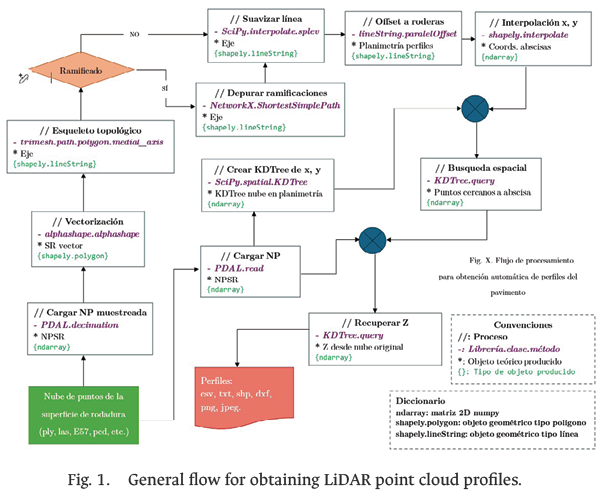, Humberto Ramírez-Gómez2 , Wilmar Fernandez-Gomez3

1 [email protected], 2 [email protected]:, 3 [email protected]

13 Sustainable Infrastructure Research Group, Universidad Distrital Francisco José de Caldas, Colombia |

2 Bogota's Special Administrative Unit for Bogota Road Rehabilitation and Maintenance

Recibido: 05 Mayo 2025 / Publicado: 24 Abril 2026
https://doi.org/10.26439/ciic2025.8669

Abstract—Pavement Management Systems integrate advanced decision-making tools for road management. This research addresses the automated approach for analyzing the light detection and ranging (LiDAR) data for road management. The proposed framework integrates machine learning techniques with advanced data-processing methodologies to estimate the International Roughness Index (IRI) using mobile LiDAR measurements. The data were obtained from the publicly available Lille2 and IQmulus point-cloud datasets, captured using the L3D2 mobile mapping systems. Automatic extraction of the rolling surface was performed on these datasets, enabling the subsequent automated generation of pavement profiles. In addition, the layout of edges, axes and profiles was automated. These alignments provided the corresponding Z-coordinates required for IRI computation, enabling faster and more accurate calculations. For both clouds, the differences observed in the global IRI values calculated from averaged reference profiles are small—ranging from 0.15 to 0.29 m/km for Lille2 and from 0.03 to 0.04 m/km for IQmulus. In contrast, the differences between these values and the IRI obtained from profiles generated using the simple method are substantially larger, ranging from 8.98 to 11.59 m/km for Lille2 and from 0.47 to 0.65 m/km for IQmulus. The results of this work will not only contribute to academic development in this field, but also to the practical implementation of more modern, efficient, and accurate systems for road network assessment and maintenance.

Index Terms—International Roughness Index (IRI), mobile LiDAR, pavements,
point clouds, road surface.

Thematic Axes—Construction processes and new technologies.

1. Introduction

In countries such as the United States, New Zealand and Canada, the public road infrastructure sector benefited from management systems developed in the private sector and subsequently began to identify ways in which public administrations could adopt the best practices of private enterprise [1]. In this context, the concept of Transportation Asset Management Systems (TAMS) emerged. When applied to road infrastructure, these systems are commonly referred to as Highway Management Systems. According to the Transportation Asset Management Subcommittee of the American Association of State Highway and Transportation Officials (AASHTO), Transportation Asset Management is defined as a strategic and systematic process that encompasses the operation, maintenance, improvement, and expansion of assets throughout their life cycle. It is grounded in business and engineering practices aimed at optimizing resource allocation. Its purpose is to ensure efficient decision-making based on quality information and clearly defined objectives, thereby maximizing asset value and performance over time.

The Transportation Asset Management Guide states that “transportation asset management is a strategic and systematic process for the operation, maintenance, updating and expansion of physical assets effectively throughout their life cycle [2]. It concentrates on business and engineering practices for the allocation and use of resources, with the objective of enabling better decision making based on high-quality data and clearly defined objectives.” However, in general terms, a road administration manages typical assets such as physical infrastructure (e.g., pavements and bridges); human resources (including personnel and technical expertise); equipment and materials; and other valuable elements such as rights of way, data, computer systems, methods and technologies.

The decision-making framework for road management should be guided by asset performance targets over an extended period, i.e., with a long-term planning and analysis horizon [1]. Performance is defined as the degree to which an asset serves its users and fulfills intended purposes, measured in terms of the quality and duration of the cumulative service it provides. In other words, performance can be described as the combination of the quality of service provided by the asset and the duration of its useful life.

A. Road infrastructure inventories

The road infrastructure inventory is used to determine the operational and functional conditions of a roadway based on a detailed description of its physical, geometric, and design conditions. The most common method for compiling this inventory is visual inspection, which consists of surveying the sector or section under study to quantify and assess its conditions. The methodology for the visual inspection includes a complete description of three fundamental aspects: (1) road description; (2) road geometry; and (3) the pavement surface condition and complementary works.

A road description consists of recording its general characteristics, including location, direction of travel, boundaries, road type (highway, arterial, collector road, and local road), and pavement type (flexible, surface treatment, rigid, and gravel or dirt). Among the criteria that must be examined in road geometry are section length, roadway width, number of lanes, shoulder width and height, median strip, and shoulder areas. The visibility distance and braking distance available may also be analyzed. Evaluating the surface condition of the pavement involves identifying flaws, defects, or damage that compromise performance and may shorten its useful life.

The evaluation of the condition of urban roads and highways is a critical aspect of analyzing operational factors related to the infrastructure’s quality and level of service. The condition of road infrastructure influences the macroscopic parameters of volume, speed, and density considered in the study of traffic phenomena. This is explained by the fact that, depending on the road’s geometric characteristics, pavement condition, and associated structures, users (drivers and pedestrians) determine their preferences when making any trip. This, in turn, affects vehicular and pedestrian flow behavior, the speeds achieved by vehicles, and the outcomes of the analysis performed on the values obtained for the aforementioned parameters [3].

B. International Roughness Index (IRI)

To define the IRI, a mathematical model is used that simulates the suspension and masses of a typical vehicle traveling along a section of road at a given speed. This model is known by its English acronym, QCS (Quarter Car Simulation), as it represents a quarter of a four-wheeled vehicle or a single-wheel trailer. The IRI at a point on a roadway is defined as the ratio of the relative movement accumulated by the suspension of a typical vehicle, to the distance traveled by that vehicle. If the longitudinal road profile, y (x) , and the car speed, V , are known, the movement, z1 and z2 , of the masses, m1 and m2 , that make up the model can be calculated at each point.

In turn, the vehicle’s response can be expressed in terms of the rectified slope (RS), at each point where the longitudinal profile is discretized.

where, z1 and z2 represent the gradients of the vehicle masses at different positions, i, along the wheel path. Finally, the IRI is obtained as the arithmetic mean of the rectified gradient along the path traveled. Therefore,

where n is the number of points counted.

It is obvious that a vehicle’s dynamic response while traveling on a roadway, and consequently its IRI value, strongly depends on the vehicle’s operating speed. To resolve this ambiguity, and after weighing the various alternatives, the International Road Roughness Experiment (IRRE) participants established 80 km/h as the reference speed for defining the IRI. This speed was chosen because the IRI coefficients obtained at this speed were considered representative of the safety and comfort perceived by users. Furthermore, this speed was deemed suitable for measurement using response-type systems.

To calculate the IRI, it is necessary to know the slopes z’1 and z’2 of the masses of the typical vehicle at each point along a section. These slopes are obtained recursively, based on the values calculated in the previous point. Thus, if the vehicle’s motion at point i-1 is known, the response at the next point can be calculated using the equation:

where {Z}= [Z 2 ‘, Z 2 ”, Z 1 ‘, Z 1 ”] T , with primes representing spatial derivatives, and represents the distance between samples, is constant within each interval, dx , and [ST] and [RS] are 4 x 4 and 4x1 matrices, respectively, whose coefficients depend on the sample interval, dx. The above system of equations can be solved for any point on the road, except for the first point of the first section where the values of zi ‘, z2 ‘, zi ” and z2 ” at the previous point are unknown. The above procedure for calculating the IRI is valid for intervals between measurements, dx, between 0.25 and 0.6 m horizontally. For shorter intervals, it is recommended to smooth the longitudinal profile to more accurately represent how a vehicle’s wheel traverses the roadway section. For this purpose, either the equivalent profile is determined every 0.25 m. (ignoring intermediate points), or a running average calculated at each point with a smoothing interval of 0.25 m. In the first case, the IRI is calculated using 0.25 m intervals, and in the second case, it is calculated using the original interval, but with the smoothed profile [4].

C. Light Detection and Ranging (LiDAR)

LiDAR is a remote sensing method that uses a laser to measure distances. A laser scanner emits pulses of light, and when a pulse strikes a target, a portion of its photons is reflected back to the scanner. Because the scanner’s position, the pulse’s direction, and the time between emission and return are known, the three-dimensional (3D) location (XYZ coordinates) from which the pulse is reflected can be calculated. The laser emits millions of such pulses and records their reflections, generating a highly accurate 3D point cloud (model) that can be used to estimate the 3D structure of the target area. Most often, the scanning laser is mounted on an aircraft—usually a fixed-wing aircraft, although increasingly on drones—and scans the terrain along its flight path. Scanning lasers are also mounted on a tripod or vehicle for terrestrial laser scanning (TLS).

A pulse is the emission produced by the scanning laser. It can be considered a time-stamped group of photons. When the pulse strikes a target, some of its photons are reflected back and detected by the LiDAR system, indicating that an echo has been received. Therefore, the source of an echo is a location struck by a pulse from which photons are reflected. An emitted pulse can, and often does, produce multiple echoes. LiDAR data contains information for each echo that is received. For example, in a text format (.txt), the data are often structured so that each row contains the information associated with a single echo, including its XYZ coordinates, intensity, and order when multiple echoes are present. Most often, LiDAR data comes in a compressed LAS/LAZ format. The LAS format is a standard file format for LiDAR data storage, where the LAZ format is a compressed format of LAS. The compressed LAZ file may be as small as 50 MB, but when decompressed and converted to a text file—often containing tens of millions of rows (one per echo)—its size can reach several GB. There are many specialized programs designed to process and analyze LiDAR data, and most common remote sensing and geographic information system (GIS) programs can also process LiDAR data in LAS/LAZ format.

Mobile LiDAR, defined as the 3D data acquisition system mounted on ground vehicles, is an advanced technology that enables high-resolution geospatial information to be captured efficiently and accurately [5]. This system has transformed road infrastructure surveys and analyses by offering a modern and automated alternative to traditional methods such as profilometers or static levelling.

2. Data and Methods

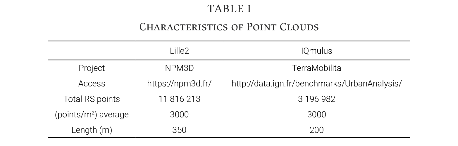
Pavement profiles were obtained from two freely accessible point clouds: Lille2 [6] and IQmulus [7]. These were captured with the L3D2 [8] and Stereopolis II [9] mobile mapping systems ADDIN CSL_CITATION {"citationitems":[{"id":"ITEM-1","item Data":{"ISSN":"17689791","abstract": "Precise realistic models of outdoor environments such as cities and roads are useful for various applications. However, achieving a high level of detail over a large environment requires addressing the challenges of the volume of data to be acquired, processed and stored, as well as the overall processing time. This paper introduces an integrated on-board laser range sensing system designed to address this need. It is intended to perform geometric modeling of urban and road environments during movement. It is based on a laser range sensor mounted on a vehicle whose position is known using GPS-INS localization. It generates raw 3D range data and performs specific modelling for cities and features extraction for roads.","author":[{"dropping particle":"","family":"Goulette","given":"F","non dropping particle":"","parse names":false,"suffix":""},{"dropping particle":"","family":"Nashashibi","given":"F","non dropping particle":"","parse names":false,"suffix":""},{"dropping particle":"","family":"Abuhadrous","given":"I","non dropping particle":"","parse names":false,"suffix":""},{"dropping particle":"","family":"Ammoun","given":"S","non dropping particle":"","parse names":false,"suffix":""},{"dropping particle":"","family":"Laurgeau","given":"C","non dropping particle":"","parse names":false,"suffix":""}],"container title":"Revue Francaise de Photogrammetrie et de Teledetection","id":"ITEM 1","issue":"185","issued":{"date parts":[["2007"]]},"page":"78 83","title":"An integrated on-board laser range sensing system for on-the-way city and road modelling","type":"article journal"},"uris":["http://www.mendeley.com/documents/?uuid=f1726048 40e1 3665 93b1 5ba3ef1a458d"]}],"mendeley":{"formattedCitation":"[8]","plainTextFormattedCitation":"[8]","previouslyFormattedCitation":"[8]"},"properties":{"noteindex":0},"schema":"https://github.com/citation style language/schema/raw/master/csl citation.json"}, respectively. The most important information from these point clouds is summarized in Table I.

The experiments were carried out on a system equipped with an Intel Core i7-10750H CPU at 2.60 GHz, running Windows 11, with 32 GB of DDR4 RAM and a 6 GB NVIDIA GeForce GTX 1660 Ti GPU. The Python language was used for all development and experimentation, utilizing environment virtualization with Conda.

Obtaining a profile requires determining the topographic coordinates x, y, z of each point spaced 25 cm along the rut alignment. To achieve this automatically, the workflow presented in Fig. 1 must be followed. The general flow of this phase includes the following steps: vectorizing the rolling surface point cloud (RSPC), calculating the topological skeleton of the road, calculating the planimetric coordinates for each abscissa of the profile, retrieving the Z coordinate of each abscissa. The vectorization of the rolling surface converts the point cloud into a planimetric polygon for processing in advanced geometric models. This procedure, common in LiDAR data processing, involves converting coordinates into two-dimensional representations using techniques such as α-shapes [10]. It was implemented using the Python α-shape library with Shapely for handling geospatial data and PDAL for loading the point cloud in NumPy format. To optimize processing, data reduction was applied with the PDAL decimation method, minimizing the number of points without compromising the road geometry.

The topological skeleton, calculated with the Trimesh library, allows extraction of the road corridor’s median axis using the medial_axis method, based on Voronoi diagrams [11]. In urban networks, it is necessary to eliminate branches, which was solved with NetworkX using Shortest_Simple_Path to extract the optimal trajectory from the skeleton. To improve the regularity of the horizontal alignment, smoothing was applied with SciPy’s splev function, generating a B-spline interpolation on the calculated trajectory. Then, the planimetric coordinates of the profiles were obtained with Shapely’s parallel_offset, ensuring their alignment with the tire marks.

Z coordinate retrieval was performed using a KD-tree, an efficient search structure implemented with SciPy. Three strategies were compared: nearest point mapping (NN), averaging the nearest 50 points (K50), and averaging points within a 10 cm radius (QB10). These techniques enabled accurate extraction of the 3D geometry of road profiles, facilitating the calculation of the IRI. The combination of these methodologies and tools facilitated progress towards the automation of road data processing, optimizing infrastructure assessment and maintenance.

From the complete point cloud, the RSPC must be classified and obtained. Using this, the rut lines corresponding to the alignment of the vehicle tire trajectory are obtained, which in this study are referred to as profiles. For Lille2, the four rut profiles were calculated and for IQmulus, two rut profiles were computed. For both scenarios, a Δx of 0.25 m was used and in each case, three iterations were performed corresponding to the three methods for estimating the Z coordinate. The location of the tire tracks was defined based on the dimensions of each corridor and assuming an average vehicle width equal to 1.8 m. In the case of Lille2, the road is 8 m wide for two lanes, so the centerline offsets were set at 1.1 m and 2.9 m to the right and left, respectively. The IQmulus cloud has a single 3.5 m wide lane, with track locations set 0.9 m on either side of the median axis. Fig. 2 shows the location of each track profile on the road surface in vector format.

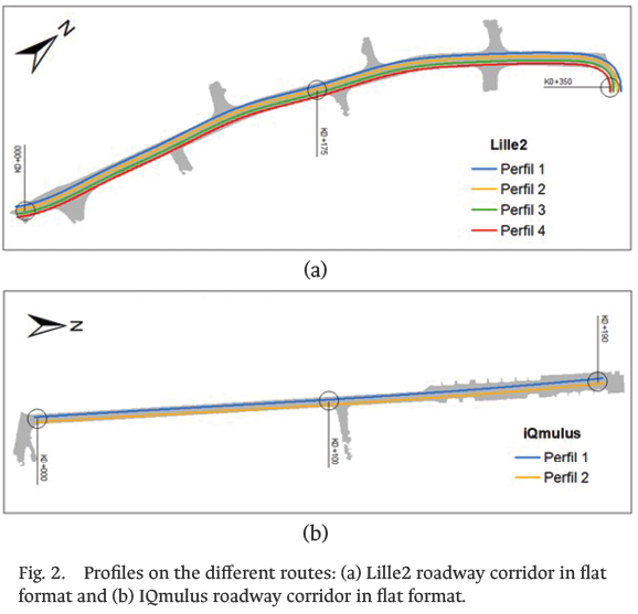
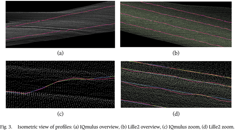
Fig. 3 shows an isometric view of the profiles. This shows the level of detail that can be collected with mobile LiDAR sensors, demonstrating that this technology provides a high-precision 3D representation, which is equivalent to, and even superior to, the information obtained through conventional topography [12]. Consequently, the profiles obtained from mobile LiDAR point clouds can be considered true profiles of the pavement and are therefore suitable for calculating the IRI, as this index corresponds to a property [13]. According to NCHRP Report 748 [14], for pavement regularity analysis, a LiDAR point cloud suitable for such analyses must have a density greater than 1000 points/m2. It is also recommended that the sampling range for estimating the vertical component be between 2 and 10 cm.

Fig. 3 also shows the profiles directly from the point clouds allowing visualization of the discrepancies between the geometries obtained by the different methods. In both cases, the pink profile, corresponding to the one obtained using the nearest Z, exhibits more irregular behavior due to the peaks in both the upper and lower sections. In contrast, the profiles generated with the other two methods maintain a smoother and more consistent trajectory, to the extent that the green and blue profiles effectively merge into a single line.

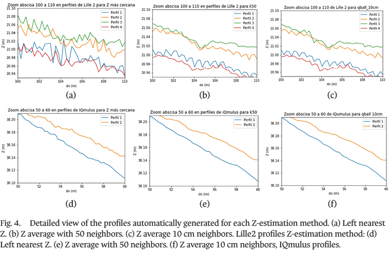
A more detailed view of the profiles, suitable for a more precise analysis of the results, is presented in Fig. 4. This figure provides a zoomed-in view of the profiles obtained with each Z-axis estimation method over two abscissas separated by only 10 m. This figure confirms the previously described divergences in the profile geometries, as well as the more irregular behavior observed in the profiles derived from the nearest-neighbor Z-axis estimation.

3. Results and Discussion

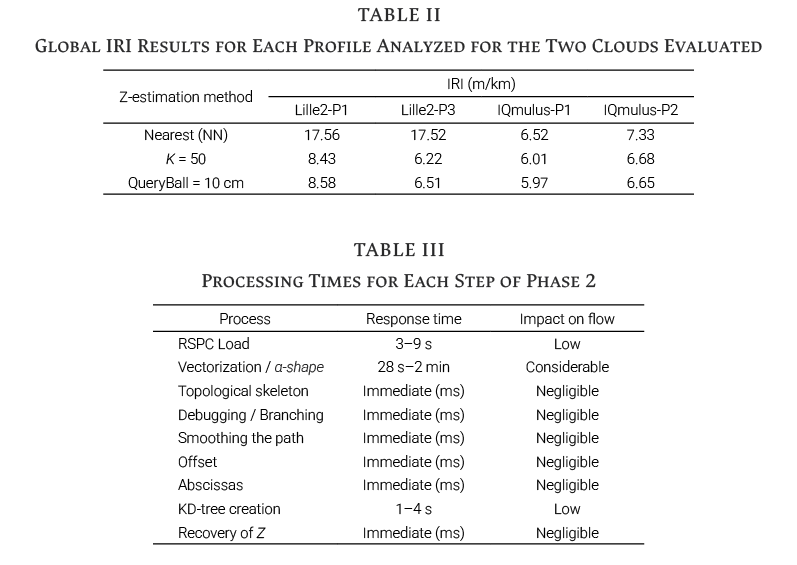
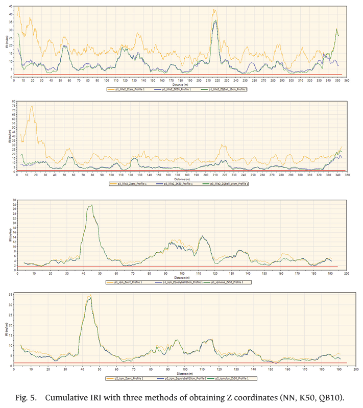
For the analysis and discussion, the IRIs of profiles 1 and 3 (corresponding to the external and internal wheel paths of different lanes) from the Lille2 dataset, as well as the two profiles from the IQmulus dataset were calculated using ProVAL software. The IRI results for each Z-estimation method for these profiles are presented in Table II below.

While Table II shows the total IRI for each profile, Fig. 5 exhibits the accumulated IRI on each abscissa for each profile, with the three different methods for obtaining Z. As evidenced by this table and figure, the relationship described in the profiles section remains consistent: the methods that estimate the Z value using multiple neighboring points yield similar results, whereas the nearest-neighbor method produces noticeably more divergent outcomes.

On the other hand, it should be noted that the implementation of the proposed methodology showed that the only step in this phase that requires substantial computational resources is the calculation of the concave envelope. For the other steps, the execution times are negligible, ranging from milliseconds to seconds. For IQmulus, the concave envelope calculation time was 28 s, and for Lille2, it was 2 min. Table III shows the times and their impact on the proposed workflow. It can also be observed that the profile calculation takes approximately 2 min for clouds containing up to 11,000,000 points, such as Lille2.

The clouds used in this experiment meet the suggested density as shown in Table III. The Z-retrieval method with a 10 cm radius also meets the proposed sampling range. The Z-retrieval method based on the 50 nearest neighbors approaches this range, exceeding it by 3 cm, as it reaches a total of 13 cm in all directions when considering the point-cloud density. In this context, the point clouds used and the profiles obtained with elevation-retrieval methods from multiple points are, in principle, suitable for pavement regularity analysis, since both methods produce highly similar profiles. This suggests that a slight increase in the proposed sampling range does not significantly affect the results.

On the other hand, an analysis of the vertical accuracy of the point clouds would be necessary, which is suggested to be submillimeter, according to the same report. This accuracy is typically assessed by comparing the elevations obtained from the point clouds with those measured through topographic leveling. However, the documentation for the clouds used does not reflect this procedure, so this criterion cannot be taken into account in this discussion.

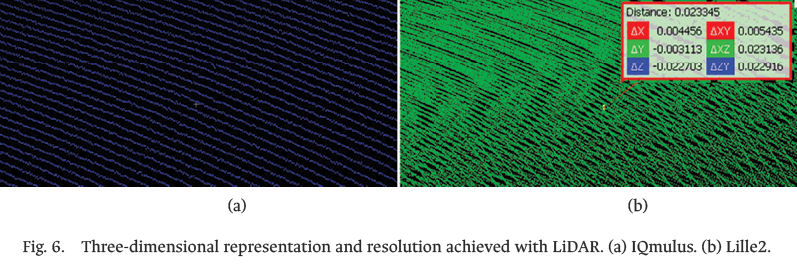
A qualitative analysis of the geometric characteristics of the point clouds indicates that, in the case of IQmulus, the cloud exhibits greater geometric consistency in its representation, due to the visibly ordered and coherent scan lines, as shown in Fig. 6(a). In contrast, the Lille2 point cloud contains scan lines that intersect without maintaining coherence in the recorded elevations. As shown in Fig. 6(b), two points separated by only 5 mm in planimetric distance (∆XY) exhibit a vertical difference (∆Z) of 2 cm, meaning they are practically in the same horizontal position.

The scenario depicted in Fig. 6(b) occurs repeatedly throughout the Lille2 RSPC, indicating that this point cloud does not adequately represent the pavement surface. It could be hypothesized that this issue arises from a mismatch between the GNSS/IMU positioning module and the LiDAR system; However, the documentation available for the cloud [6], [8] is insufficient to draw a conclusive diagnosis, and therefore the cause of this situation remains unknown. A primary guideline to consider when extracting pavement profiles from mobile LiDAR data is the geometric coherence of the point cloud. This experimentation allows for the distinction of two potential scenarios. On one hand, a geometrically coherent point cloud, as is the case with IQmulus, in which the heights of the scan lines are adjusted to reality, without presenting different elevations for the same position. On the other hand, the opposite case is the Lille2 point cloud, where different elevations are recorded at the same location.

The implemented methodology formulates a strategy to handle geometrically inconsistent point clouds by calculating the Z value based on the average of multiple nearby reference points. These methods also yield more robust and reliable results when applied to geometrically coherent point clouds, compared to those obtained using a simple Z calculation based solely on the nearest reference point.

A comparison of the Lille2 profiles shows that the methods based on averaged reference points effectively smooth the resulting profile relative to that obtained using the simple nearest-point method. However, the resulting profiles still exhibit a behavior that is too erratic for a paved surface, indicating that true profiles were not obtained due to the geometric inconsistency of the RSPC. This suggests that the proposed methods are not sufficient to handle this type of cloud, and that new strategies would be required for this purpose or, ultimately, to discard this type of cloud from profile calculations.

For IQmulus profiles, it is again observed that the multi-reference averaged methods smooth the profile calculated with the simple method. In this case, however, all methods yield a similar pavement profile due to the geometric coherence of the cloud. In accordance with the above, and given that the RSPCs meet the recommended point density, it can be stated that the profiles computed for IQmulus correspond to the true pavement profiles and that, consequently, the IRIs derived from them are theoretically correct. However, their practical validation cannot be carried out, as this would only be possible by comparing the results with profiles obtained through well-established methods, such as topography or high-speed inertial profilometers. This validation is beyond the scope of this research. Nevertheless, the results demonstrate that this methodology can generate suitable products to be used as inputs in the calculation of this index through specialized software, such as ProVAL.

Although it cannot be confirmed that the IRIs calculated from the IQmulus data match those obtained using well-established methods, the results highlight relevant aspects regarding the influence of the Z coordinate calculation method on this index. For both clouds, the differences between the global IRIs (Table II), calculated using averaged reference profiles, are small: between 0.15 and 0.29 m/km for Lille2, and between 0.03 and 0.04 m/km for IQmulus. In contrast, the differences between these same values and the IRIs obtained with profiles calculated using the simple method are significantly greater: between 8.98 and 11.59 m/km for Lille2, and between 0.47 and 0.65 m/km for IQmulus.

It is then evident that the simple Z-retrieval method increases the IRI from magnitudes in the cm range to values above 8 m/km in the case of Lille2, and from magnitudes in the mm range to values greater than 0.4 m/km in the case of IQmulus. This trend can also be seen in the accumulated IRI graphs, where the orange profiles always remain above the other two profiles, while the latter almost always maintain the same trajectory. This indicates that calculating the IRI from profiles obtained using simple methods is not reliable because these approaches assume very abrupt relative elevation changes. These arise because in many cases the heights obtained are not truly representative of the regions to which the abscissas belong, but instead correspond by chance to the nearest points. It is therefore acknowledged that the most appropriate approach is always to use a Z recovery method that considers multiple height references, thereby avoiding the reporting of inflated IRI values, which in many cases could lead to unnecessary pavement interventions.

On the other hand, the results show that the implemented workflow allows recreating pavement profiles in a short time. It should be noted that no references in the available literature propose a method to automate the extraction of pavement profiles. The study most closely related to this work is presented in [15], where the correlation between IRIs obtained from mobile LiDAR and those obtained from high-speed inertial profilometers is reviewed. It was demonstrated that a high correlation exists between these measurements, and that the potential to quantify the regularity of the entire surface is greater than when using linear profile measurements alone.

The research focused on comparing both technologies without dedicating much effort to automating the procedure. Z recovery was performed by reconstructing Digital Elevation Models (DEM) with two different interpolation methods, Inverse Distance Weighting (IDW) and Kriging. This resulted in processing times of 30 min and 10 h, respectively, for a cloud of 150,000,000 points representing 4 km of track. Considering that, in both the aforementioned research and this study, profile calculation only requires coordinate information (X, Y, Z), it is valid to establish a processing time per point relationship. Using this, the method in [15] would require between 0.012 and 0.24 ms of processing per point to obtain the surface from which the ordinates and abscissas of the profile are extracted, whereas the methodology proposed here requires approximately 0.011 ms per point to obtain the complete profile.

In that order, this methodology presents a marginal advantage over the analyzed method, but, in addition, it contributes new elements to the field of LiDAR processing automation for road management, allowing to automatically obtain the axis and the edges of the road, which are objects of study with considerable research interest, as reflected in the works of [16], [17], [18]. Likewise, in this work, the concepts, ordered steps and possible technologies (Python, in this case) for the implementation of the workflow are exhaustively detailed, so that it can be easily understood, improved and reproduced by other researchers in the area. Faced with this, the results show that the proposed processing flow is highly computationally efficient, since the profiles are obtained in a few seconds except for the step of vectorizing the RSPC that requires the calculation of α-shape , increasing the processing time due to the high algorithmic complexity of this technique [19].

4. Conclusions

A methodology has been established for the automatic extraction of pavement profiles from mobile LiDAR data, and its effectiveness has been demonstrated in accomplishing two essential tasks: the extraction of road edges and centerlines, and the recovery of Z values for the abscissas defining each axis.

The high level of detail and accuracy provided by mobile LiDAR enables the resulting profiles to accurately represent the true pavement profile, thereby facilitating direct IRI calculations.

The results obtained demonstrate the viability of the proposed methodology. First, an effective elevation data recovery strategy from mobile LiDAR scenes enables accurate recreation of the true pavement profile. Second, the proposed processing workflow for automatic profile generation is highly computationally efficient, as most products are obtained within seconds, except for the RSPC vectorization step, which requires the computation of α-shapes, thereby increasing processing time due to the high algorithmic complexity of this technique.

5. References

   [1] Federal Highway Administration, Asset Management Overview, FHWA-IF-08-008, U.S. Department of Transportation, Office of Asset Management, Washington, D.C., Dec. 2007. [Online]. Available: https://www.fhwa.dot.gov/asset/if08008/assetmgmt_overview.pdf?

   [2] American Association of State Highway and Transportation Officials (AASHTO), Transportation Asset Management Guide: A Focus on Implementation, 2nd ed., ch. 1, “Introduction” (secs. 1.1–1.3). Washington, D.C.: AASHTO, Feb. 27, 2020. [Online]. Available: https://www.tamguide.com/wp-content/uploads/2020/02/TAM_GuideIII_ch01-20200227.pdf?

   [3] J. R. Quintero González, “Inventarios viales y categorización de la red vial en estudios de Ingeniería de Tránsito y Transporte,” Revista Facultad de Ingeniería, UPTC, vol. 20, no. 30, pp. 65–77, 2011. [Online]. Available: https://dialnet.unirioja.es/descarga/articulo/3758451.pdf

   [4] M. W. Sayers, “On the Calculation of International Roughness Index from Longitudinal Road Profile,” Transportation Research Record: Journal of the Transportation Research Board, no. 1501, pp. 1–12, 1995. [Online]. Available: http://onlinepubs.trb.org/Onlinepubs/trr/1995/1501/1501-001.pdf

   [5] K. Williams, M. Olsen, G. Roe, and C. Glennie, “Synthesis of Transportation Applications of Mobile LIDAR,” Remote Sensing, vol. 5, no. 9, pp. 4652–4692, Sep. 2013, doi: https://doi.org/10.3390/rs5094652

   [6] X. Roynard, J.-E. Deschaud, and F. Goulette, “Paris-Lille-3D: A large and high-quality ground-truth urban point cloud dataset for automatic segmentation and classification,” The International Journal of Robotics Research, vol. 37, no. 6, pp. 545–557, Apr. 2018, doi: https://doi.org/10.1177/0278364918767506

   [7] B. Vallet, M. Brédif, A. Serna, B. Marcotegui, and N. Paparoditis, “TerraMobilita/iQmulus urban point cloud analysis benchmark,” Computers & Graphics, vol. 49, pp. 126–133, Jun. 2015, doi: https://doi.org/10.1016/j.cag.2015.03.004

   [8] F. Goulette, F. Nashashibi, I. Abuhadrous, S. Ammoun, and C. Laurgeau, “An integrated on-board laser range sensing system for on-the-way city and road modeling,” Revue Française de Photogrammétrie et de Télédétection, no. 185, pp. 78-83, 2007.

   [9] N. Paparoditis et al., “Stereopolis II: A multi-purpose and multi-sensor 3D mobile mapping system for street visualisation and 3D metrology,” Revue française de photogrammétrie et de télédétection, no. 200, pp. 69–79, Apr. 2014, doi: https://doi.org/10.52638/rfpt.2012.63

   [10] H. Edelsbrunner, D. Kirkpatrick, and R. Seidel, “On the shape of a set of points in the plane,” IEEE Transactions on Information Theory, vol. 29, no. 4, pp. 551–559, Jul. 1983, doi: https://doi.org/10.1109/tit.1983.1056714

   [11] F. P. Preparata and M. I. Shamos, Computational Geometry: An Introduction, New York / Berlin / Heidelberg: Springer, 1985. doi: https://doi.org/10.1007/978-1-4612-1098-6

   [12] T. Křemen, M. Štroner, and P. Třasák, “Determination of Pavement Elevations by the 3D Scanning System and Its Verification,” Geoinformatics FCE CTU, vol. 12, pp. 55–60, Jun. 2014, doi: https://doi.org/10.14311/gi.12.9

   [13] M. W. Sayers and S. M. Karamihas, The Little Book of Profiling: Basic Information about Measuring and Interpreting Road Profiles, Ann Arbor, MI: University of Michigan Transportation Research Institute, Sep. 1998. [Online]. Available: https://hdl.handle.net/2027.42/21605

   [14] M. J. Olsen et al., Guidelines for the Use of Mobile LiDAR in Transportation Applications, NCHRP Report 748, Transportation Research Board, Washington, D.C., 2013. [Online]. Available: https://onlinepubs.trb.org/onlinepubs/nchrp/nchrp_rpt_748.pdf

   [15] M. R. De Blasiis, A. Di Benedetto, M. Fiani, and M. Garozzo, “Assessing of the Road Pavement Roughness by Means of LiDAR Technology,” Coatings, vol. 11, no. 1, Art. no. 17, Dec. 2020, doi: https://doi.org/10.3390/coatings11010017

   [16] B. Suleymanoglu, M. Soycan, and C. Toth, “3D Road Boundary Extraction Based on Machine Learning Strategy Using LiDAR and Image-Derived MMS Point Clouds,” Sensors, vol. 24, no. 2, Art. no. 503, Jan. 2024, doi: https://doi.org/10.3390/s24020503

   [17] Y. Wang et al., “Framework for Geometric Information Extraction and Digital Modeling from LiDAR Data of Road Scenarios,” Remote Sensing, vol. 15, no. 3,
   Art. no. 576, Jan. 2023, doi: https://doi.org/10.3390/rs15030576

   [18] J. Wang, X. Dong, and G. Liu, “Extraction of Urban Road Boundary Points from Mobile Laser Scanning Data Based on Cuboid Voxel,” ISPRS International Journal of Geo-Information, vol. 12, no. 10, Art. no. 426, Oct. 2023, doi: https://doi.org/10.3390/ijgi12100426

   [19] Z. Yahya, R. W. Rahmat, F. Khalid, A. Rizaan, and A. Rizal, “A Concave Hull Based Algorithm for Object Shape Reconstruction,” International Journal of Information Technology and Computer Science, vol. 9, no. 3, pp. 1–9, Mar. 2017, doi: https://doi.org/10.5815/ijitcs.2017.03.01